Data Infrastructure

• 1: Unified Namespace
• 2: Historian / Data Storage
• 3: Shopfloor KPIs / Analytics (v1)
• 3.1: Shopfloor KPIs / Analytics (v0)
• 4: Alerting

1 - Unified Namespace

The Unified Namespace is a centralized, standardized, event-driven data architecture that enables for seamless integration and communication across various devices and systems in an industrial environment. It operates on the principle that all data, regardless of whether there is an immediate consumer, should be published and made available for consumption. This means that any node in the network can work as either a producer or a consumer, depending on the needs of the system at any given time.

This architecture is the foundation of the United Manufacturing Hub, and you can read more about it in the Learning Hub article.

When should I use it?

In our opinion, the Unified Namespace provides the best tradeoff for connecting systems in manufacturing / shopfloor scenarios. It effectively eliminates the complexity of spaghetti diagrams and enables real-time data processing.

While data can be shared through databases, REST APIs, or message brokers, we believe that a message broker approach is most suitable for most manufacturing applications. Consequently, every piece of information within the United Manufacturing Hub is transmitted via a message broker.

Both MQTT and Kafka are used in the United Manufacturing Hub. MQTT is designed for the safe message delivery between devices and simplifies gathering data on the shopfloor. However, it is not designed for reliable stream processing. Although Kafka does not provide a simple way to collect data, it is suitable for contextualizing and processing data. Therefore, we are combining both the strengths of MQTT and Kafka. You can get more information from this article.

What can I do with it?

The Unified Namespace in the United Manufacturing Hub provides you the following functionalities and applications:

• Seamless Integration with MQTT: Facilitates straightforward connection with modern industrial equipment using the MQTT protocol.
• Legacy Equipment Compatibility: Provides easy integration with older systems using tools like Node-RED or Benthos UMH, supporting various protocols like Siemens S7, OPC-UA, and Modbus.
• Real-time Notifications: Enables instant alerting and data transmission through MQTT, crucial for time-sensitive operations.
• Historical Data Access: Offers the ability to view and analyze past messages stored in Kafka logs, which is essential for troubleshooting and understanding historical trends.
• Scalable Message Processing: Designed to handle a large amount of data from a lot of devices efficiently, ensuring reliable message delivery even over unstable network connections. By using IT standard tools, we can theoretically process data in the measure of GB/second instead of messages/second.
• Data Transformation and Transfer: Utilizes the Data Bridge to adapt and transmit data between different formats and systems, maintaining data consistency and reliability.

Each feature opens up possibilities for enhanced data management, real-time monitoring, and system optimization in industrial settings.

You can view the Unified Namespace by using the Management Console like in the picture below. The picture shows data under the topic umh/v1/demo-pharma-enterprise/Cologne/_historian/rainfall/isRaining, where

• umh/v1 is a versioning prefix.
• demo-pharma-enterprise is a sample enterprise tag.
• Cologne is a sample site tag.
• _historian is a schema tag. Data with this tag will be stored in the UMH’s database.
• rainfall/isRaining is a sample schema dependent context, where rainfall is a tag group and isRaining is a tag belonging to it.

The full tag name uniquely identifies a single tag, it can be found in the Publisher & Subscriber Info table.

The above image showcases the Tag Browser, our main tool for navigating the Unified Namespace. It includes the following features:

• Data Aggregation: Automatically consolidates data from all connected instances / brokers.
• Topic Structure: Displays the hierarchical structure of topics and which data belongs to which namespace.
• Tag Folder Structure: Facilitates browsing through tag folders or groups within a single asset.
• Schema validation: Introduces validation for known schemas such as _historian. In case of validation failure, the corresponding errors are displayed.
• Tag Error Tracing: Enables error tracing within the Unified Namespace tree. When errors are detected in tags or schemas, all affected nodes are highlighted with warnings, making it easier to track down the troubled source tags or schemas.
• Publisher & Subscriber Info: Provides various details, such as the origins and destinations of the data, the instance it was published from, the messages per minute to get an overview on how much data is flowing, and the full tag name to uniquely identify the selected tag.
• Payload Visualization: Displays payloads under validated schemas in a formatted/structured manner, enhancing readability. For unknown schemas without strict validation, the raw payload is displayed instead.
• Tag Value History: Shows the last 100 received values for the selected tag, allowing you to track the changes in the data over time. Keep in mind that this feature is only available for tags that are part of the _historian schema.
• Example SQL Query: Generates example SQL queries based on the selected tag, which can be used to query the data in the UMH’s database or in Grafana for visualization purposes.
• Kafka Origin: Provides information about the Kafka key, topic and the actual payload that was sent via Kafka.

It’s important to note that data displayed in the Tag Browser represent snapshots; hence, data sent at intervals shorter than 10 seconds may not be accurately reflected.

You can find more detailed information about the topic structure here.

You can also use tools like MQTT Explorer (not included in the UMH) or Redpanda Console (enabled by defualt, accessible via port 8090) to view data from a single instance (but single instance only).

How can I use it?

To effectively use the Unified Namespace in the United Manufacturing Hub, start by configuring your IoT devices to communicate with the UMH’s MQTT broker, considering the necessary security protocols. While MQTT is recommended for gathering data on the shopfloor, you can send messages to Kafka as well.

Once the devices are set up, handle the incoming data messages using tools like Node-RED or Benthos UMH. This step involves adjusting payloads and topics as needed. It’s also important to understand and follow the ISA95 standard model for data organization, using JSON as the primary format.

Additionally, the Data Bridge microservice plays a crucial role in transferring and transforming data between MQTT and Kafka, ensuring that it adheres to the UMH data model. You can configure a merge point to consolidate messages from multiple MQTT topics into a single Kafka topic. For instance, if you set a merge point of 3, the Data Bridge will consolidate messages from more detailed topics like umh/v1/plant1/machineA/temperature into a broader topic like umh/v1/plant1. This process helps in organizing and managing data efficiently, ensuring that messages are grouped logically while retaining key information for each topic in the Kafka message key.

Recommendation: Send messages from IoT devices via MQTT and then work in Kafka only.

What are the limitations?

While JSON is the only supported payload format due to its accessibility, it’s important to note that it can be more resource-intensive compared to formats like Protobuf or Avro.

Where to get more information?

• Explore the UMH architecture and data model.
• Read articles about MQTT, Kafka, and the Unified Namespace on the Learning Hub.
• Read the blog article about Tools & Techniques for scalable data processing in Industrial IoT.

2 - Historian / Data Storage

The Historian / Data Storage feature in the United Manufacturing Hub provides reliable data storage and analysis for your manufacturing data. Essentially, a Historian is just another term for a data storage system, designed specifically for time-series data in manufacturing.

When should I use it?

If you want to reliably store data from your shop floor that is not designed to fulfill any legal purposes, such as GxP, we recommend you to use the United Manufacturing Hub’s Historian feature. In our opinion, open-source databases such as TimescaleDB are superior to traditional historians in terms of reliability, scalability and maintainability, but can be challenging to use for the OT engineer. The United Manufacturing Hub fills this usability gap, allowing OT engineers to easily ingest, process, and store data permanently in an open-source database.

What can I do with it?

The Historian / Data Storage feature of the United Manufacturing Hub allows you to:

Store and analyze data

• Store data in TimescaleDB by using either the _historian or _analytics _schemas in the topics within the Unified Namespace.
• Data can be sent to the Unified Namespace from various sources, allowing you to store tags from your PLC and production lines reliably. Optionally, you can use tag groups to manage a large number of tags and reduce the system load. Our Data Model page assists you in learning data modeling in the Unified Namespace.
• Conduct basic data analysis, including automatic downsampling, gap filling, and statistical functions such as Min, Max, and Avg.

Query and visualize data

• Query data in an ISA95 compliant model, from enterprise to site, area, production line, and work cell.
• Visualize your data in Grafana to easily monitor and troubleshoot your production processes.

More information about the exact analytics functionalities can be found in the umh-datasource-v2 documentation.

Efficiently manage data

• Compress and retain data to reduce database size using various techniques.

How can I use it?

To store your data in TimescaleDB, simply use the _historian or _analytics _schemas in your Data Model v1 compliant topic. This can be directly done in the OPC UA data source when the data is first inserted into the stack. Alternatively, it can be handled in Node-RED, which is useful if you’re still utilizing the old data model, or if you’re gathering data from non-OPC UA sources via Node-RED or sensorconnect.

Data sent with a different _schema will not be stored in TimescaleDB.

Data stored in TimescaleDB can be viewed in Grafana. An example can be found in the Get Started guide.

In Grafana you can select tags by using SQL queries. Here, you see an example:

SELECT name, value, timestamp
FROM tag
WHERE asset_id = get_asset_id(
  'pharma-genix',
  'aachen',
  'packaging',
  'packaging_1',
  'blister'
);

get_asset_id is a custom plpgsql function that we provide to simplify the process of querying tag data from a specific asset. To learn more about our database, visit this page.

Also, you have the option to query data in your custom code by utilizing the API in factoryinsight or processing the data in the Unified Namespace.

For more information about what exactly is behind the Historian feature, check out our our architecture page.

What are the limitations?

• In order to store messages, you should transform data and use our topic structure. The payload must be in JSON using a specific format, and the message must be tagged with _historian.
• After storing a couple of millions messages, you should consider compressing the messages or establishing retention policies.

Apart from these limitations, the United Manufacturing Hub’s Historian feature is highly performant compared to legacy Historians.

Where to get more information?

• Learn more about the benefits of using open-source databases in our blog article, Historians vs Open-Source databases - which is better?
• Check out the Getting Started guide to start using the Historian feature.
• Learn more about the United Manufacturing Hub’s architecture by visiting our architecture page.
• Learn more about our Data Model by visiting this page.
• Learn more about our database for _historian schema by visiting our documentation.

3 - Shopfloor KPIs / Analytics (v1)

The Shopfloor KPI / Analytics feature of the United Manufacturing Hub provides a configurable and plug-and-play approach to create “Shopfloor Dashboards” for production transparency consisting of various KPIs and drill-downs.

Click on the images to enlarge them. More examples can be found in this YouTube video and in our community-repo on GitHub.

When should I use it?

If you want to create production dashboards that are highly configurable and can drill down into specific KPIs, the Shopfloor KPI / Analytics feature of the United Manufacturing Hub is an ideal choice. This feature is designed to help you quickly and easily create dashboards that provide a clear view of your shop floor performance.

What can I do with it?

The Shopfloor KPI / Analytics feature of the United Manufacturing Hub allows you to:

Query and visualize

In Grafana, you can:

• Calculate the OEE (Overall Equipment Effectiveness) and view trends over time
  • Availability is calculated using the formula (plannedTime - stopTime) / plannedTime, where plannedTime is the duration of time for all machines states that do not belong in the Availability or Performance category, and stopTime is the duration of all machine states configured to be an availability stop.
  • Performance is calculated using the formula runningTime / (runningTime + stopTime), where runningTime is the duration of all machine states that consider the machine to be running, and stopTime is the duration of all machine states that are considered a performance loss. Note that this formula does not take into account losses caused by letting the machine run at a lower speed than possible. To approximate this, you can use the LowSpeedThresholdInPcsPerHour configuration option (see further below).
  • Quality is calculated using the formula good pieces / total pieces
• Drill down into stop reasons (including histograms) to identify the root-causes for a potentially low OEE.
• List all produced and planned orders including target vs actual produced pieces, total production time, stop reasons per order, and more using job and product tables.
• See machine states, shifts, and orders on timelines to get a clear view of what happened during a specific time range.
• View production speed and produced pieces over time.

Configure

In the database, you can configure:

• Stop Reasons Configuration: Configure which stop reasons belong into which category for the OEE calculation and whether they should be included in the OEE calculation at all. For instance, some companies define changeovers as availability losses, some as performance losses. You can easily move them into the correct category.
• Automatic Detection and Classification: Configure whether to automatically detect/classify certain types of machine states and stops:
  • AutomaticallyIdentifyChangeovers: If the machine state was an unspecified machine stop (UnknownStop), but an order was recently started, the time between the start of the order until the machine state turns to running, will be considered a Changeover Preparation State (10010). If this happens at the end of the order, it will be a Changeover Post-processing State (10020).
  • MicrostopDurationInSeconds: If an unspecified stop (UnknownStop) has a duration smaller than a configurable threshold (e.g., 120 seconds), it will be considered a Microstop State (50000) instead. Some companies put small unknown stops into a different category (performance) than larger unknown stops, which usually land up in the availability loss bucket.
  • IgnoreMicrostopUnderThisDurationInSeconds: In some cases, the machine can actually stop for a couple of seconds in routine intervals, which might be unwanted as it makes analysis difficult. One can set a threshold to ignore microstops that are smaller than a configurable threshold (usually like 1-2 seconds).
  • MinimumRunningTimeInSeconds: Same logic if the machine is running for a couple of seconds only. With this configurable threshold, small run-times can be ignored. These can happen, for example, during the changeover phase.
  • ThresholdForNoShiftsConsideredBreakInSeconds: If no shift was planned, an UnknownStop will always be classified as a NoShift state. Some companies move smaller NoShift’s into their category called “Break” and move them either into Availability or Performance.
  • LowSpeedThresholdInPcsPerHour: For a simplified performance calculation, a threshold can be set, and if the machine has a lower speed than this, it could be considered a LowSpeedState and could be categorized into the performance loss bucket.
• Language Configuration: The language of the machine states can be configured using the languageCode configuration option (or overwritten in Grafana).

You can find the configuration options in the configurationTable

How can I use it?

Using it is very easy:

1. Send messages according to the UMH datamodel to the Unified Namespace (similar to the Historian feature)
2. Configure your OEE calculation by adjusting the configuration table
3. Open Grafana, and checkout our tutorial on how to select the data.

For more information about what exactly is behind the Analytics feature, check out our architecture page and our datamodel

Where to get more information?

• Learn more about the benefits of using open-source databases in our blog article, Historians vs Open-Source databases - which is better?
• Learn more about the United Manufacturing Hub’s architecture by visiting our architecture page.
• Learn more about the datamodel by visiting our datamodel
• To build visual dashboards, check out our tutorial on using Grafana Canvas

3.1 - Shopfloor KPIs / Analytics (v0)

The Shopfloor KPI / Analytics feature of the United Manufacturing Hub provides a configurable and plug-and-play approach to create “Shopfloor Dashboards” for production transparency consisting of various KPIs and drill-downs.

When should I use it?

If you want to create production dashboards that are highly configurable and can drill down into specific KPIs, the Shopfloor KPI / Analytics feature of the United Manufacturing Hub is an ideal choice. This feature is designed to help you quickly and easily create dashboards that provide a clear view of your shop floor performance.

What can I do with it?

The Shopfloor KPI / Analytics feature of the United Manufacturing Hub allows you to:

Query and visualize

In Grafana, you can:

• Calculate the OEE (Overall Equipment Effectiveness) and view trends over time
  • Availability is calculated using the formula (plannedTime - stopTime) / plannedTime, where plannedTime is the duration of time for all machines states that do not belong in the Availability or Performance category, and stopTime is the duration of all machine states configured to be an availability stop.
  • Performance is calculated using the formula runningTime / (runningTime + stopTime), where runningTime is the duration of all machine states that consider the machine to be running, and stopTime is the duration of all machine states that are considered a performance loss. Note that this formula does not take into account losses caused by letting the machine run at a lower speed than possible. To approximate this, you can use the LowSpeedThresholdInPcsPerHour configuration option (see further below).
  • Quality is calculated using the formula good pieces / total pieces
• Drill down into stop reasons (including histograms) to identify the root-causes for a potentially low OEE.
• List all produced and planned orders including target vs actual produced pieces, total production time, stop reasons per order, and more using job and product tables.
• See machine states, shifts, and orders on timelines to get a clear view of what happened during a specific time range.
• View production speed and produced pieces over time.

Configure

In the database, you can configure:

• Stop Reasons Configuration: Configure which stop reasons belong into which category for the OEE calculation and whether they should be included in the OEE calculation at all. For instance, some companies define changeovers as availability losses, some as performance losses. You can easily move them into the correct category.
• Automatic Detection and Classification: Configure whether to automatically detect/classify certain types of machine states and stops:
  • AutomaticallyIdentifyChangeovers: If the machine state was an unspecified machine stop (UnknownStop), but an order was recently started, the time between the start of the order until the machine state turns to running, will be considered a Changeover Preparation State (10010). If this happens at the end of the order, it will be a Changeover Post-processing State (10020).
  • MicrostopDurationInSeconds: If an unspecified stop (UnknownStop) has a duration smaller than a configurable threshold (e.g., 120 seconds), it will be considered a Microstop State (50000) instead. Some companies put small unknown stops into a different category (performance) than larger unknown stops, which usually land up in the availability loss bucket.
  • IgnoreMicrostopUnderThisDurationInSeconds: In some cases, the machine can actually stop for a couple of seconds in routine intervals, which might be unwanted as it makes analysis difficult. One can set a threshold to ignore microstops that are smaller than a configurable threshold (usually like 1-2 seconds).
  • MinimumRunningTimeInSeconds: Same logic if the machine is running for a couple of seconds only. With this configurable threshold, small run-times can be ignored. These can happen, for example, during the changeover phase.
  • ThresholdForNoShiftsConsideredBreakInSeconds: If no shift was planned, an UnknownStop will always be classified as a NoShift state. Some companies move smaller NoShift’s into their category called “Break” and move them either into Availability or Performance.
  • LowSpeedThresholdInPcsPerHour: For a simplified performance calculation, a threshold can be set, and if the machine has a lower speed than this, it could be considered a LowSpeedState and could be categorized into the performance loss bucket.
• Language Configuration: The language of the machine states can be configured using the languageCode configuration option (or overwritten in Grafana).

You can find the configuration options in the configurationTable

How can I use it?

Using it is very easy:

1. Send messages according to the UMH datamodel to the Unified Namespace (similar to the Historian feature)
2. Configure your OEE calculation by adjusting the configuration table
3. Open Grafana, select your equipment and select the analysis you want to have. More information can be found in the umh-datasource-v2.

For more information about what exactly is behind the Analytics feature, check out our our architecture page and our datamodel

What are the limitations?

At the moment, the limitations are:

• Speed losses in Performance are not calculated and can only be approximated using the LowSpeedThresholdInPcsPerHour configuration option
• There is no way of tracking losses through reworked products. Either a product is scrapped or not.

Where to get more information?

• Learn more about the benefits of using open-source databases in our blog article, Historians vs Open-Source databases - which is better?
• Learn more about the United Manufacturing Hub’s architecture by visiting our architecture page.
• Learn more about the datamodel by visiting our datamodel
• To build visual dashboards, check out our tutorial on using Grafana Canvas

4 - Alerting

The United Manufacturing Hub utilizes a TimescaleDB database, which is based on PostgreSQL. Therefore, you can use the PostgreSQL plugin in Grafana to implement and configure alerts and notifications.

Why should I use it?

Alerts based on real-time data enable proactive problem detection. For example, you will receive a notification if the temperature of machine oil or an electrical component of a production line exceeds limitations. By utilizing such alerts, you can schedule maintenance, enhance efficiency, and reduce downtime in your factories.

What can I do with it?

Grafana alerts help you keep an eye on your production and manufacturing processes. By setting up alerts, you can quickly identify problems, ensuring smooth operations and high-quality products. An example of using alerts is the tracking of the temperature of an industrial oven. If the temperature goes too high or too low, you will get an alert, and the responsible team can take action before any damage occurs. Alerts can be configured in many different ways, for example, to set off an alarm if a maximum is reached once or if it exceeds a limit when averaged over a time period. It is also possible to include several values to create an alert, for example if a temperature surpasses a limit and/or the concentration of a component is too low. Notifications can be sent simultaneously across many services like Discord, Mail, Slack, Webhook, Telegram, or Microsoft Teams. It is also possible to forward the alert with SMS over a personal Webhook. A complete list can be found on the Grafana page about alerting.

How can I use it?

Follow this tutorial to set up an alert.

Alert Rule

When creating an alert, you first have to set the alert rule in Grafana. Here you set a name, specify which values are used for the rule, and when the rule is fired. Additionally, you can add labels for your rules, to link them to the correct contact points. You have to use SQL to select the desired values.

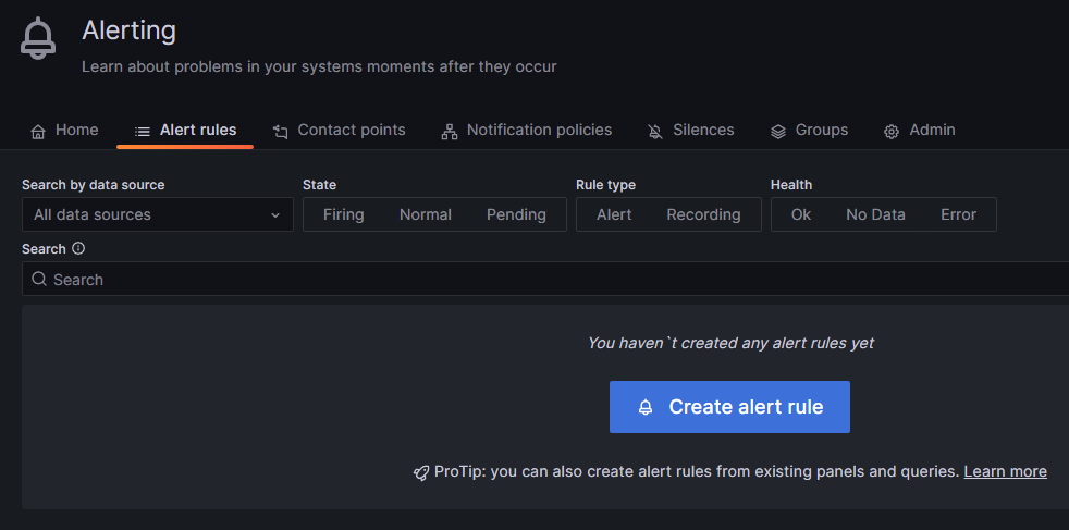
1. To add a new rule, hover over the bell symbol on the left and click on Alert rules. Then click on the blue Create alert rule button.

   

   

2. Choose a name for your rule.

3. In the next step, you need to select and manipulate the value that triggers your alert and declare the function for the alert.

• Subsection A is, by default the selection of your values: You can use the Grafana builder for this, but it is not useful, as it cannot select a time interval even though there is a selector for it. If you choose, for example, the last 20 seconds, your query will select values from hours ago. Therefore, it is necessary to use SQL directly. To add command manually, switch to Code in the right corner of the section.

  • First, you must select the value you want to create an alert for. In the United Manufacturing Hub’s data structure, a process value is stored in the table tag. Unfortunately Grafana cannot differentiate between different values of the same sensor; if you select the ConcentrationNH3 value from the example and more than one of the selected values violates your rule in the selected time interval, it will trigger multiple alerts. Because Grafana is not able to tell the alerts apart, this results in errors. To solve this, you need to add the value "timestamp" to the Select part. So the first part of the SQL command is: SELECT value, "timestamp".
  • The source is tag, so add FROM tag at the end.
  • The different values are distinguished by the variable name in the tag, so add WHERE name = '<key-name>' to select only the value you need. If you followed Get Started guide, you can use temperature as the name.
  • Since the selection of the time interval in Grafana is not working, you must add this manually as an addition to the WHERE command: AND "timestamp" > (NOW() - INTERVAL 'X seconds'). X is the number of past seconds you want to query. It’s not useful to set X to less than 10 seconds, as this is the fastest interval Grafana can check your rule, and you might miss values.

  The complete command is:

  SELECT value, "timestamp" FROM tag WHERE name = 'temperature' AND "timestamp" > (NOW() - INTERVAL '10 seconds')
  

• In subsection B, you need to reduce the values to numbers, Grafana can work with. By default, Reduce will already be selected. However, you can change it to a different option by clicking the pencil icon next to the letter B. For this example, we will create an upper limit. So selecting Max as the Function is the best choice. Set Input as A (the output of the first section) and choose Strict for the Mode. So subsection B will output the maximum value the query in A selects as a single number.

• In subsection C, you can establish the rule. If you select Math, you can utilize expressions like $B > 120 to trigger an alert when a value from section B ($B means the output from section B) exceeds 50. In this case, only the largest value selected in A is passed through the reduce function from B to C. A simpler way to set such a limit is by choosing Threshold instead of Math.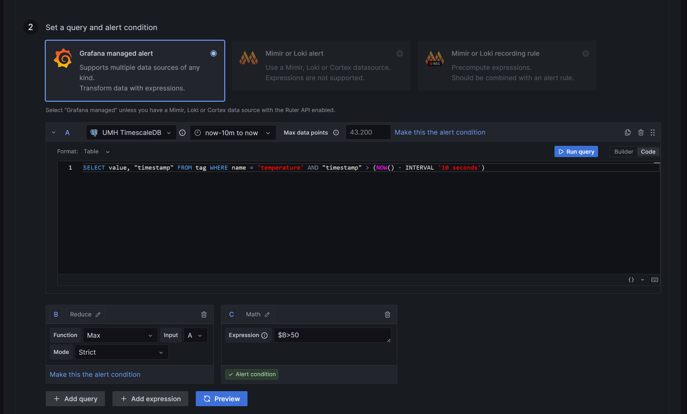

  

  

  To add more queries or expressions, find the buttons at the end of section two and click on the desired option. You can also preview the results of your queries and functions by clicking on Preview and check if they function correctly and fire an alert.

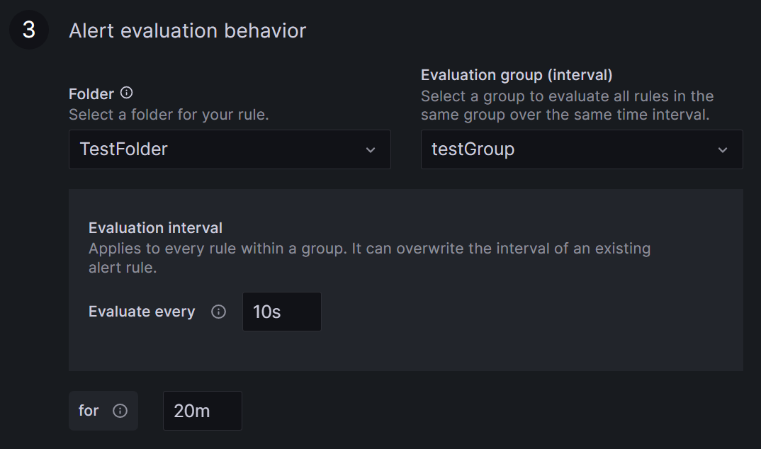
4. Define the rule location, the time interval for rule checking, and the duration for which the rule has to be broken before an alert is triggered.

   • Select a name for your rule’s folder or add it to an existing one by clicking the arrow. Find all your rules grouped in these folders on the Alert rules page under Alerting.

   • An Evaluation group is a grouping of rules, which are checked after the same time interval. Creating a new group requires setting a time interval for rule checking. The minimum interval from Grafana is ten seconds.

   • Specify the duration the rule must be violated before triggering the alert. For example, with a ten-second check interval and a 20-second duration, the rule must be broken twice in a row before an alert is fired.

     

     

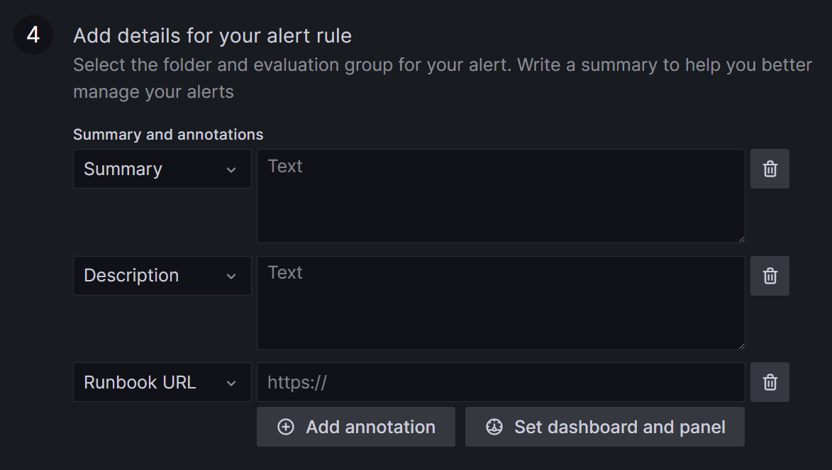
5. Add details and descriptions for your rule.

   

   

6. In the next step, you will be required to assign labels to your alert, ensuring it is directed to the appropriate contacts. For example, you may designate a label team with alertrule1: team = operator and alertrule2: team = management. It can be helpful to use labels more than once, like alertrule3: team = operator, to link multiple alerts to a contact point at once.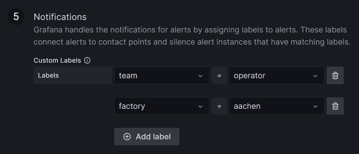

   

   

Your rule is now completed; click on Save and Exit on the right upper corner, next to section one.

Contact Point

In a contact point you create a collection of addresses and services that should be notified in case of an alert. This could be a Discord channel or Slack for example. When a linked alert is triggered, everyone within the contact point receives a message. The messages can be preconfigured and are specific to every service or contact. The following steps shall be done to create a contact point.

1. Navigate to Contact points, located at the top of the Grafana alerting page.

2. Click on the blue + Add contact point button.

3. Now, you should be able to see setting page. Choose a name for your contact point.

   

   

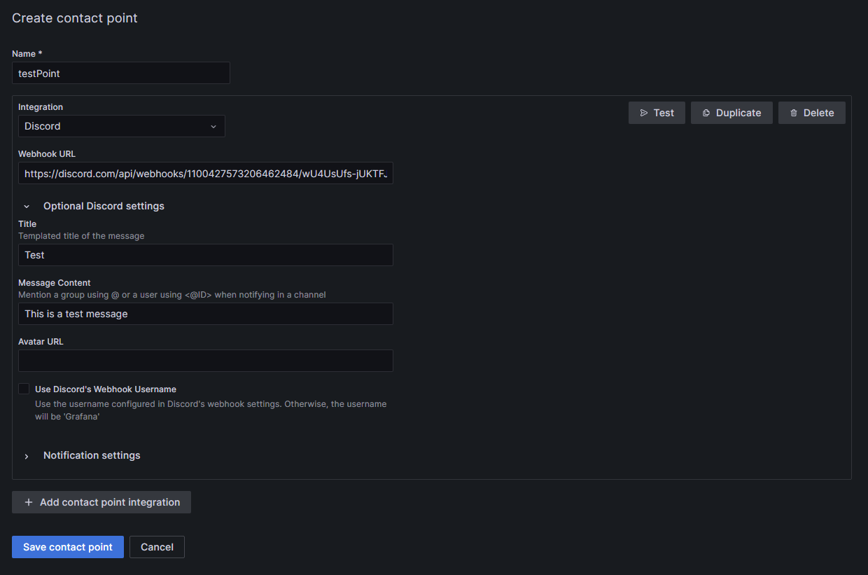
4. Pick the receiving service; in this example, Discord.

5. Generate a new Webhook in your Discord server (Server Settings ⇒ Integrations ⇒ View Webhooks ⇒ New Webhook or create Webhook). Assign a name to the Webhook and designate the messaging channel. Copy the Webhook URL from Discord and insert it into the corresponding field in Grafana. Customize the message to Discord under Optional Discord settings if desired.

6. If you need, add more services to the contact point, by clicking + Add contact point integration.

7. Save the contact point; you can see it in the Contact points list, below the grafana-default-email contact point.

Notification Policies

In a notification policy, you establish the connection of a contact point with the desired alerts. To add the notification policy, you need to do the following steps.

1. Go to the Notification policies section in the Grafana alerting page, next to the Contact points.

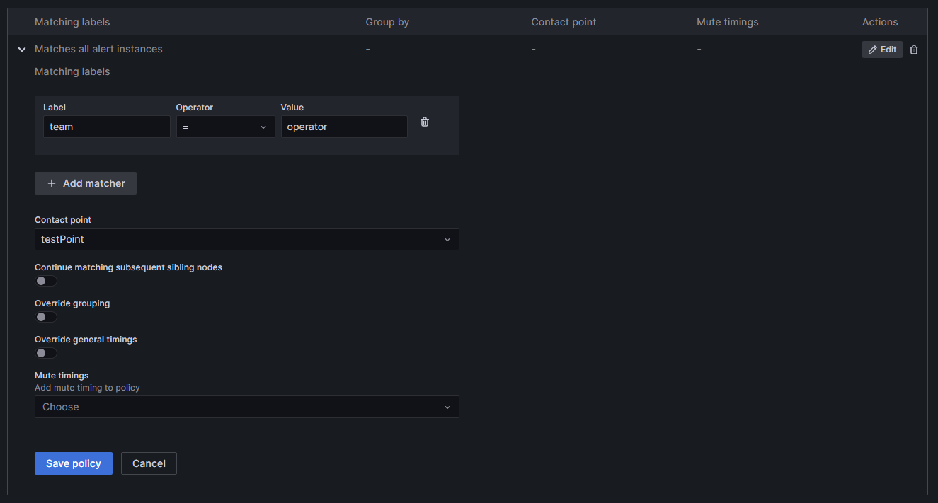
2. Select + New specific policy to create a new policy, followed by + Add matcher to choose the label and value from the alert (for example team = operator). In this example, both alert1 and alert3 will be forwarded to the associated contact point. You can include multiple labels in a single notification policy.

3. Choose the contact point designated to receive the alert notifications. Now, the inputs should be like in the picture.

   

   

4. Press Save policy to finalize your settings. Your new policy will now be displayed in the list.

Mute Timing

In case you do not want to receive messages during a recurring time period, you can add a mute timing to Grafana. You can set up a mute timing in the Notification policies section.

1. Select + Add mute timing below the notification policies.

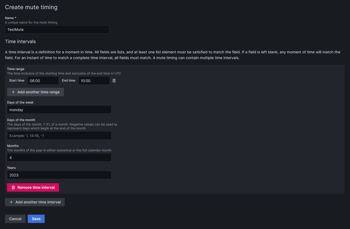
2. Choose a name for the mute timing.

3. Specify the time during which notifications should not be forwarded.

   • Time has to be given in UTC time and formatted as HH:MM. Use 06:00 instead of 6:00 to avoid an error in Grafana.

4. You can combine several time intervals into one mute timing by clicking on the + Add another time interval button at the end of the page.

5. Click Submit to save your settings.

6. To apply the mute timing to a notification policy, click Edit on the right side of the notification policy, and then select the desired mute timing from the drop-down menu at the bottom of the policy. Click on Save Policy to apply the change.

   

   

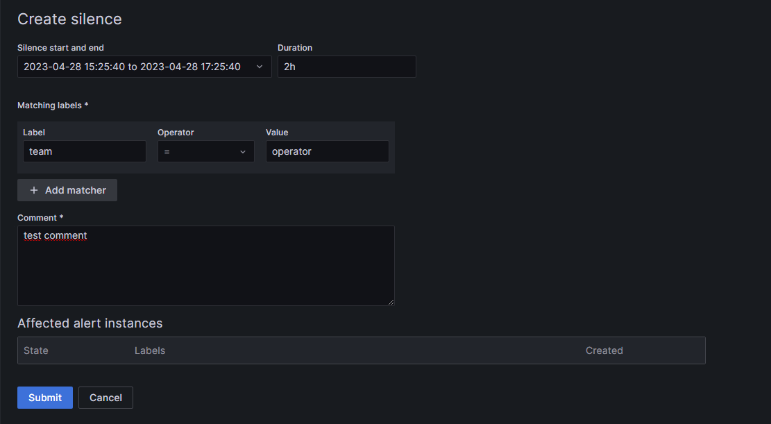
Silence

You can also add silences for a specific time frame and labels, in case you only want to mute alerts once. To add a silence, switch to the Silences section, next to Notification policies.

1. Click on + Add Silence.

2. Specify the beginning for the silence and its duration.

3. Select the labels and their values you want silenced.

4. If you need, you can add a comment to the silence.

5. Click the Submit button at the bottom of the page.

   

   

What are the limitations?

It can be complicated to select and manipulate the desired values to create the correct function for your application. Grafana cannot differentiate between data points of the same source. For example, you want to make a temperature threshold based on a single sensor. If your query selects the last three values and two of them are above the threshold, Grafana will fire two alerts which it cannot tell apart. This results in errors. You have to configure the rule to reduce the selected values to only one per source to avoid this. It can be complicated to create such a specific rule with this limitation, and it requires some testing.

Another thing to keep in mind is that the alerts can only work with data from the database. It also does not work with the machine status; these values only exist in a raw, unprocessed form in TimescaleDB and are not processed through an API like process values.

Where to get more information?

• The Grafana page about alerting
• How to add Grafana to Teams